Remote-Sensing Derived Trends in Gross Primary Production Explain Increases in the CO₂ Seasonal Cycle Amplitude

L. He^1,2, B. Byrne³, Y. Yin¹, J. Liu⁴ and C. Frankenberg⁴

¹California Institute of Technology, Pasadena, CA 91125; 626-714-9918, E-mail: lhe@carnegiescience.edu
²Carnegie Institution for Science, Department of Global Ecology, Stanford, CA 94305
³University of Toronto, Toronto, Ontario, Canada
⁴NASA Jet Propulsion Laboratory, California Institute of Technology, Pasadena, CA 91109

An increase in the seasonal cycle amplitude (SCA) of atmospheric carbon dioxide (CO₂) since the 1960s has been observed in the Northern Hemisphere (NH). However, dominant drivers of the amplified CO₂ seasonality are still debated. In this study, we employ satellite-based remote sensing observations to track spatial and temporal changes in global gross primary production (GPP) of different vegetation types. Then, we use a state-of-art atmospheric transport model to examine whether our bottom-up estimates of ecosystem fluxes can capture the magnitude of CO₂ SCA trends at multiple surface sites. Further, we explore dominant drivers of the observed CO₂ SCA trends across different locations of sites. To our best knowledge, this paper makes the first effort to link long-term satellite remote sensing observations with ground atmospheric CO₂ measurements across the NH to explore how terrestrial carbon fluxes shape and change spatiotemporal pattern of atmospheric CO₂.

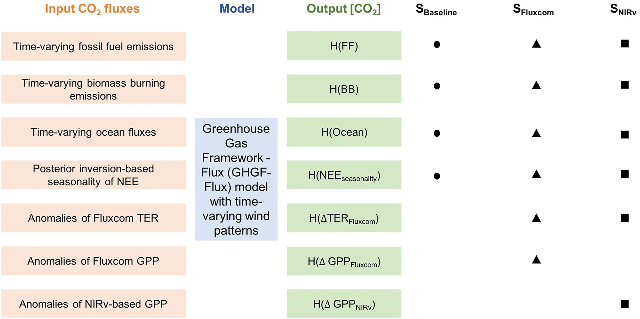
Figure 1. Diagram of the S_Baseline, S_Fluxcom, and S_NIRv simulations based on CO₂ fluxes from multiple sources. [CO₂] represents the atmospheric CO₂ concentrations. Mathematically, [CO₂] simulated in S_Baseline, S_Fluxcom, and S_NIRv can be formulated as H(FF) + H(BB) + H(Ocean) + H(NEE_seasonality), H(FF) + H(BB) + H(Ocean) + H(NEE_seasonality) + H(TER_Fluxcom) + H(GPP_Fluxcom) and H(FF) + H(BB) + H(Ocean) + H(NEE_seasonality) + H(TER_Fluxcom) + H(GPP_NIRv), where H(X) denotes the application of a forward atmospheric model to simulate CO₂ concentrations driven by fluxes X.