Introduction¶

The inversion software tries to solve the equation

(1) $\hat{s} = s_p + (HQ)^T * (HQH^T + R)^{-1} * (z-Hs_p)$

where

z is a known vector of measurements
H is a matrix that describes the relationship between measurements and the unknown fields
R is the covariance matrix of the model-data mismatch errors
s_p is the prior estimate of s
Q is a (square and symmetric) prior error covariance matrix, describing deviations between the true field s and the prior s_p.

We use the technique of Yadav and Michalak (2012) to solve this equation. Instead of creating the Q matrix directly, it is expressed instead as the Kronecker product of the temporal covariance (D) and the spatial convariance (E)

(2) $Q = \sigma_s^2 \overbrace{[ e^{(-X_\tau/l_\tau)}]}^D \otimes \overbrace{[ e^{(-X_s/l_s)}]}^E$

where $\sigma_s^2$ is the variance of the prior in space and time, X_s and X_t represent the separation distances/lags between estimation locations in space and time, respectively, and l_s and l_t are the spatial and temporal correlation range parameters, respectively.

We can use this property to calculate HQ by splitting H into p blocks, where p is the number of timesteps in the inversion, and using

(3) $HQ = \left[\left( \left( \sum_{i=1}^{p} d_{i1}h_iI_{\sigma_i}\right)EI_{\sigma_1}\right) \left( \left( \sum_{i=1}^{p} d_{i2}h_iI_{\sigma_i}\right)EI_{\sigma_2}\right) ... \left( \left( \sum_{i=1}^{p} d_{iq}h_iI_{\sigma_i}\right)EI_{\sigma_q}\right)\right]$

Note

This formula for the calculation of HQ is a modification from that described in Yadav and Michalak (Equation 9) by using a time and space varying $\sigma_s^2$ . See the section on Stage 2 - Applying Sprior sigma to H Slices and Calculating HQ

Procedure¶

The procedure for running an inversion is broken down into several stages, each involving separate data files and programs. The overall steps involved are shown in Figure 1.

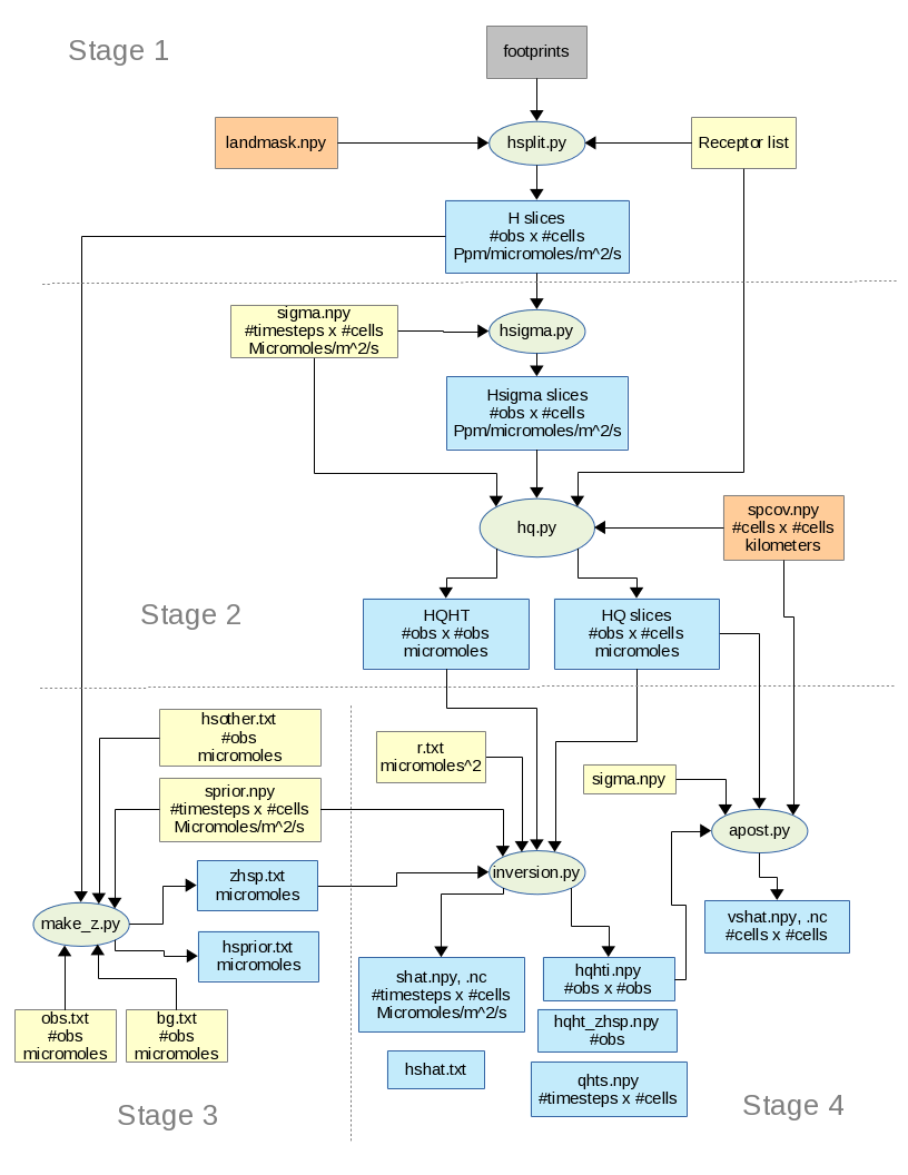
Figure 1. The green ovals are the python scripts that are used for doing the calculations in the inversions. The gray box indicates the stilt footprint files. The orange boxes indicate files that the user creates, and the file names are specified in the configuration file. The yellow boxes indicate files that the user is required to create, and the file names are given to the python scripts on the command line. The blue boxes are files that are created by the inversion scripts. Names for these are hard coded in the scripts and can not be changed by the user.

Stage 1 - Receptor list, landmask, H slice creation¶

Step 1 - Create a receptor list file.

This file contains the location of the footprint files that will be used in the inversion. One file name per line. See the section Receptor File.

Step 2 - Create configuration file.

The configuration file contains much of the information needed for the inversion, such as the physical domain, the time frame, file names to use etc. See the section Configuration File.

Step 3 - Create/specify landmask file.

Create or use a pre-made landmask file which specifies grid cells that contain land. See the section Creating a Landmask File.

Step 4 - Create H matrix slices for each timestep.

The technique involved in the inversion calculation makes use of breaking up the H matrix into smaller blocks. This step creates an H block at each timestep of the inversion from the footprint data files. See the section on Stage 1 - Creating H Slices.

Stage 2 - HQ slice creation¶

Step 1 - Create Spatial Covariance distance values.

Values for the spatical covariance matrix depend on knowning the distances between cells in the domain. This step will calculate the distances between all cells in the domain, and stores them in a numpy data file. See the section on Spatial Distances.

Step 2 - Create uncertainty values for Sprior.

The NOAA inversion code uses a modification of the Yadav and Michalak (2012) method that allows a time and space varying sigma for sprior ( $\sigma_s^2$ in equation 2). It is up to the user to create these values.

Step 3 - Apply sprior uncertainty to H slices.

Run the program hsigma.py to create new H slice files that have the sprior sigma ( $\sigma_s$ in equation 2) applied to them.

Step 4 - Create HQ slices.

Run the program hq.py to create the HQ slices at each inversion timestep, and also the $HQH^T$ term from equation 1. See the section on HQ Calculations.

Stage 3 - Prior, Observation and Background data¶

Step 1 - Create an observation value list file.

This file contains the measurement value for each footprint file in the receptor list. The lines must correspond with the receptor list lines, i.e. observation value on line 1 is for line 1 of receptor list ...

Step 2 - Create ‘background’ values.

This step determines the ‘background’ value for each receptor.

Step 3 - Create sprior and sother data.

The s_p in equation 1 is created in this step, and any additional prior values that will be subtracted from the background (such as fossil fuel, fire, ocean...)

Step 4 - Create (z-Hsp) data.

The $(z - Hs_p)$ term from equation 1 is calculated. See the section on Stage 3 - Observations, background and priors.

Stage 4 - Inversion¶

Step 1 - Create an R value list file.

This file contains a model-data mismatch value for each footprint file in the receptor list. The lines must correspond with the receptor list lines, i.e. R value on line 1 is for line 1 of receptor list ... NOTE The value on each line is the variance R²

Step 2 - Run the inversion.

Run the program inversion.py to take data created in prior stages and complete the inversion. See the section on Stage 4 - Inversion and posterior uncertainty.

Step 3 - Posterior uncertainty.

Run the program apost.py to calculate the covariance of the estimated $\hat{s}$ . See the section on Posterior uncertainty.