
GML Aerosol Measurements
Measured and Derived Aerosol Properties
In situ measurements of a variety of aerosol optical properties are being made at GML stations. The measurement suite enables calculation of direct aerosol climate forcing. The measured values relevant for climate forcing calculations are: light absorption (σap), total scattering (σsp) and hemispheric backscattering (σbsp). Additionally, most stations in the cooperative aerosol network measure total aerosol number concentration (N). The optical measurements (typically made at several wavelengths) are used to derive parameters required in the radiative forcing calculation as well as to calculate parameters which help further characterize the aerosol (e.g., by size or type) (Table 1).
Table 1: Aerosol radiative properties that can be derived from measurements made by the GML cooperative aerosol network.
| åsp (or SAE) | The scattering Ångström exponent, defined by the power-law σsp(λ)-å, describes the wavelength-dependence of scattered light. Situations where the scattering is dominated by sub-μm particles typically have values around 2, while values close to 0 occur when the scattering is dominated by particles larger than a few micrometers in diameter. |
| åap (or AAE) | The absorption Ångström exponent, defined by the power-law σap(λ)-å, describes the wavelength-dependence of light absorption. The AAE can provide indications of aerosol composition, for example, black carbon (BC), has a theoretical AAE value of 1, while dust aerosol typically has AAE values greater than 2. |
| ωo (or SSA) | The aerosol single-scattering albedo, defined as σsp/(σap+σsp), describes the relative contributions of scattering and absorption to the total light extinction. Purely scattering aerosols (e.g., sulfuric acid) have values of 1, while very strong absorbers (e.g., elemental carbon) have values around 0.3. |
| g, b, β | Radiative transfer models commonly require an integral property of the angular distribution of scattered light (phase function): the asymmetry factor g, the hemispheric backscatter fraction b, or the upscatter fraction β. The asymmetry factor is the cosine-weighted average of the phase function, ranging from a value of -1 for entirely backscattered light to +1 for entirely forward-scattered light. The hemispheric backscatter fraction b is σbsp/σsp. The upscatter fraction depends on the solar zenith angle, and is equal to b when the sun is directly overhead |
| FMF | The fine mode fraction (FMF) of aerosol light scattering (and absorption) is the ratio of sub1-μm to sub10-μm (PM1 and PM10) scattering (or absorption). Because many natural aerosols (e.g., sea salt and dust) tend to have sizes larger than 1 μm while anthropogenically-generated particles typically are sub-μm in diameter, the FMF can indicate the relative contribution of anthropogenic sources in an air mass. |
Methods
The basic GML aerosol system consists of a nephelometer (measures aerosol light scattering), an absorption photometer (a filter-based method for measuring light absorption, e.g., CLAP, aethalometer, and/or PSAP) and a condensation nuclei counter (CNC, measures particle number concentration). The measurements are typically made at two size cuts: sub10--μm and sub1--μm (PM10 and PM1). The measurements are performed at reduced relative humidity (<40%) to eliminate confounding effects due to changes in ambient relative humidity. Expanded aerosol systems may include auxilliary instrumentation such as a tandem nephelometer humidograph for measuring aerosol hygroscopicity, size distribution measurements, chemical sampling, and/or cloud condensation nuclei concentrations.
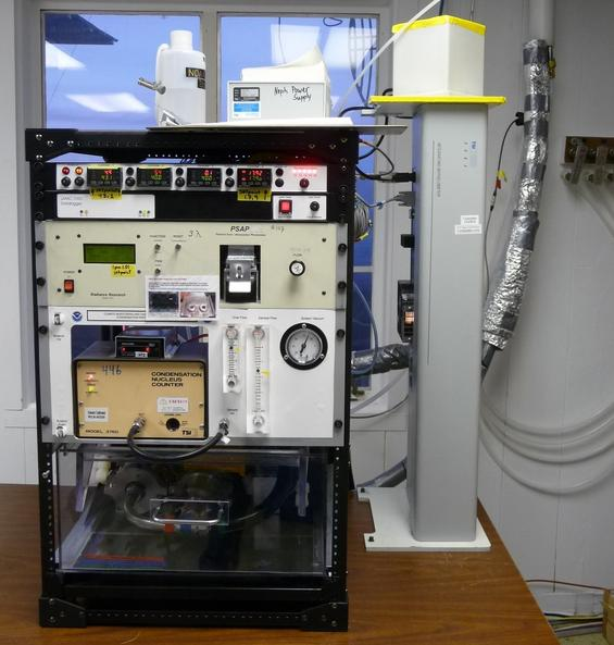
Basic Instrumentation
Page with details about the standard instruments in a basic aerosol rack system.
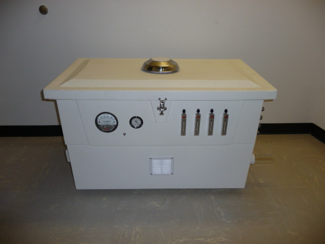
Sample Conditioning and System Control Components
Page with details about system control components (e.g., inlet, pumpbox, RH conditioning etc.)
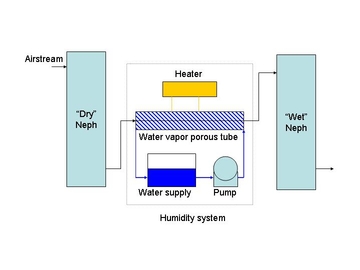
Auxilliary Instrumentation
Page with details of auxilliary instruments that have been integrated into a basic aerosol rack system.
Data Flow
The GML Aerosol group has developed software for acquisition, processing, and archiving of data from instruments used in the NOAA-federated aerosol network. This complete software package ensures data consistency among sites: Field site --> NOAA --> Site Scientist --> QC (data editing+corrections) --> WMO World Data Center for Aerosols hosted by NILU.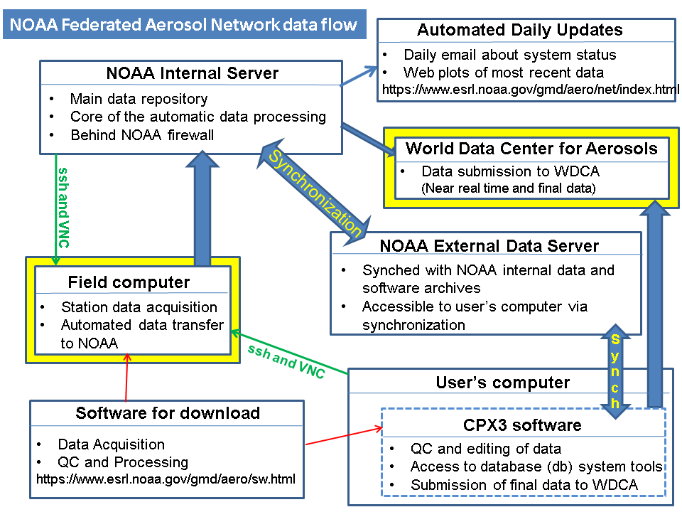
Data Treatment: Data quality control and processing
Following collection of the raw data at the station, the data undergo quality control by the system scientist. This involves inspecting the data and identifying periods of time when the measurements are invalid (i.e., due to a broken instrument or pump) or contaminated (i.e., due to non-regionally representative activity at the site such as lawn mowing). A record is kept of the data editing directives which simplifies revisiting and perhaps revising the edited data after the fact. Additionally, to generate the final data product, standard corrections are applied to the data stream. These corrections include things like the Anderson and Ogren (1998) truncation corrections to account for angular non-idealities in the nephelometer and adjustment of the data to standard temperature and pressure.
Most of the sites in the cooperative aerosol network have the goal of reporting the characteristics of regionally representative aerosol. To this end both automatic and manual contamination screening is performed. Data from the continuous sensors are screened to eliminate contamination from local pollution sources. The screening algorithms may use measured wind speed, direction, and/or total particle number concentration to flag data that are likely to have been locally contaminated. Manual screening is more subjective, relying on the station scientist to evaluate the data in the context of automated contamination flags and their knowledge about the site More information about contamination screening (both manual and automated) is found in Sheridan et al. (2016).
In order to understand the significance of trends and observed temporal cycles, it is necessary to determine the uncertainties in the measurements. The supplemental materials included with Sherman et al. (2015) describe details of the uncertainty calculations for the parameters listed in Table 1. Ogren et al., (2017) provides additional uncertainty information for the CLAP.